In a previous post we saw how to evaluate a policy and iteratively improve it. The value iteration algorithm in an alternative formalism to iteratively improve a policy. In policy iteration, we started with a random policy, evaluated the state value function, took a greedy step and iteratively updated the state value function. Here, we will start with a initial state value function and iteratively update it.

Here’s a simple sketch of the algorithm:

1. We will start with an initial value function
2. We use one_step_lookahead() from our previous example to compute the action values.
3. We will pick the action that has maximum value and update our value function. Essentially, in each iteration $k+1$, we update our value function using the value of the value function in iteration $k$, by picking the action that would fetch us the maximum value.
4. Compute the values and update until convergence.
5. Update the policy by picking the best action.

The iterative updates are achieved using Bellman Optimality equation:

Putting it together:

def value_iter(env, gamma=0.9, th=1e-9, max_iter=10000):
    # (1) initialize the value function for each state
    v = np.zeros(env.observation_space.n)
    # iterate until converges w.r.t th
    for i in range(int(max_iter)):
        # initialize change in value to 0
        delta = 0
        # for each state in environment 
        for s in range(env.observation_space.n):
            # (2) look one step ahead and compute action-value function
            action_values_vec = one_step_lookahead(env, s, v)
            # (3) select the best action value from 
            # action values from one-step lookahead
            best_val = np.max(action_values_vec)
            # calculate the change in value
            delta = max(delta, np.abs(v[s] - best_val))
            # update the value function v
            v[s] = best_val
        # check stopping condition
        if delta < th:
            print(f'\nvalue iteration converged in {i} iterations')
            break
    # create a policy 
    policy = np.zeros([env.observation_space.n, env.action_space.n])
    for s in range(env.observation_space.n):
        # look one step ahead and compute action-value function
        action_vec = one_step_lookahead(env, s, v)
        # (4) select the best action from actions from one-step lookahead
        best_a = np.argmax(action_vec)
        # update policy
        policy[s][best_a] = 1.0
    return policy, v

Policy iteration works in two phases in each iteration: 1. we evaluate the policy, 2. we improve the policy (and make updates). The value iteration combines these two phases into one. We do not explicitly evaluate a policy. Instead, we just sweep through all possible actions and find the action that leads to the best action value. Both approaches implicitly update state value function and action value function in each iteration.

As people who know me understand, I read articles and listen to podcasts on a variety of topics ranging from technology, social science, society, economics, etc. Economics is one of my favourites, as it is very relatable to our day to day lives, besides involving mathematical modelling (which, for the same reasons as Deep Learning techniques of today, can only be close to a very good approximation but never accurate). While listening to BBC’s Business Daily podcasts, I stumbled upon this episode on Modern Monetary Theory. The title of the podcast - “Magic Money Tree” caught my attention and it turned out to be an interesting take on a proposal by one of the former Hedge Fund manager about central banks being able to print more money when needed. I did have this idea when I was a kid before I realized inflation and value of goods and how they are tied to abundance of ciculation of money, interest rates and consumer spending. I am not an economist but I am worried how this could lead to powerful economies manipulating their inflation thereby leading to disastrous consequences in parts of the world whose currencies are not global trade currencies.

For those interested in listening to the episode, you can do it here:

Are there wonderful teachers among expert economists who can help me understand?

In a previous post we evaluated a given policy $\pi$ by computing the state value function $v_{\pi}(s)$ in each of the states of the system. In this post, we will start with a random policy, use the function policy_eval() developed in the previous post to improve the random policy we started with and end up in an improved policy as a result.

Recall from a previous post the intuition behind action value function.

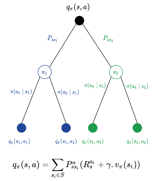
Our goal now is to do a one step lookahead and calculate the action values for different possible actions and pick the action that would fetch us the maximum action value. The following function follows the equation in the sketch above and computes action values for different possible actions.

def one_step_lookahead(env, st, v, gamma=0.9):
    action_values = np.zeros(env.action_space.n)
    for a in range(env.action_space.n):
        for nxt_st_prob, nxt_st, reward, done in env.P[st][a]:
            action_values[a] += nxt_st_prob * (reward + gamma * v[nxt_st])
    return action_values

Here is what we are going to do:

1. Start with a random policy
2. Evaluate the policy (using policy_eval()) and get the state values for all the states
3. Take one step (using one_step_lookahead()) and take the action that maximizes the action value (greedy step) and then follow our usual policy for the rest of the episode
4. Return the updated state values (resulting from one step of greedy action) along with the policy (better policy)

action_values = one_step_lookahead(env, s, v)
best_a = np.argmax(action_values)

action_values is a 4 element array (as there are four actions - Up, Down, Right and Left). The array indices indicate the action while the array elements indicate the action value ($q(s, a$)). argmax(action_values) would return the action that has the maximum action value.

Putting it all together:

def policy_iter(env, gamma=0.9, max_iter=10000):    
    # (1)  start with random policy
    policy = np.ones([env.observation_space.n, env.action_space.n]) / env.action_space.n
    # policy eval counter
    policy_eval_cnt = 1
    # repeat until convergence or max_iter
    for i in range(int(max_iter)):
        stop = False
        # (2) evaluate current policy
        v = policy_eval(policy, env)
        for s in range(env.observation_space.n):
            # current action according to our policy
            curr_a = np.argmax(policy[s])
            # (3) look one step ahead and check if curr_a is the best
            action_values = one_step_lookahead(env, s, v)
            # select best action greedily from action_values from one-step lookahead
            best_a = np.argmax(action_values)
            if (curr_a != best_a):
                stop = False
                # update the policy
                policy[s] = np.eye(env.action_space.n)[best_a]
            else: # curr_a has converged to best_a
                stop = True
        policy_eval_cnt += 1
        
        if (stop):
            # (4)  return state values and updated policy
            return policy, v

This is referred to as Policy Iteration as we iteratively improve the policy that we started with, evaluating the policy in each iteration.

In one of the previous posts we saw how to evaluate the value of a state s $v_{\pi}(s)$. In this post, we will try to implement it using OpenAI Gym. Let us recall the following image that would help us in writing our policy evaluation function.

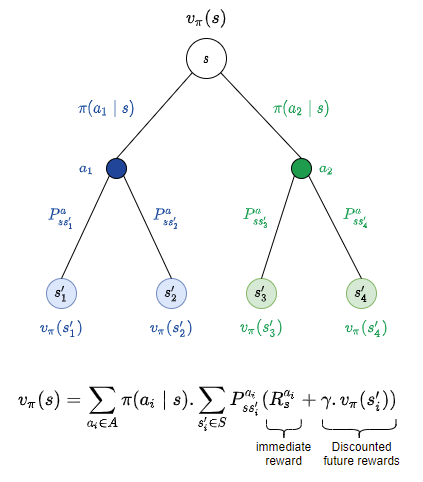
The main goal of policy evaluation is to find the state value function of the states in the system, given a policy $\pi$. To recap, for a given state $s$, there could be multiple possible actions and probabilities of each of the actions. Once we commit to an action, the environment could perform its turn of the action and our action could take us to different potential ‘next’ states, each with a probability of transition. We average over all the action probabilities $\pi(a_i \mid s)$ and over the transition probabilities $P_{ss’_{i}}^{a_i}$ and compute immediate reward and discounted rewards on next state.

The (pseudo)code fragment for the different components are given alongside the figure below for better intuition.

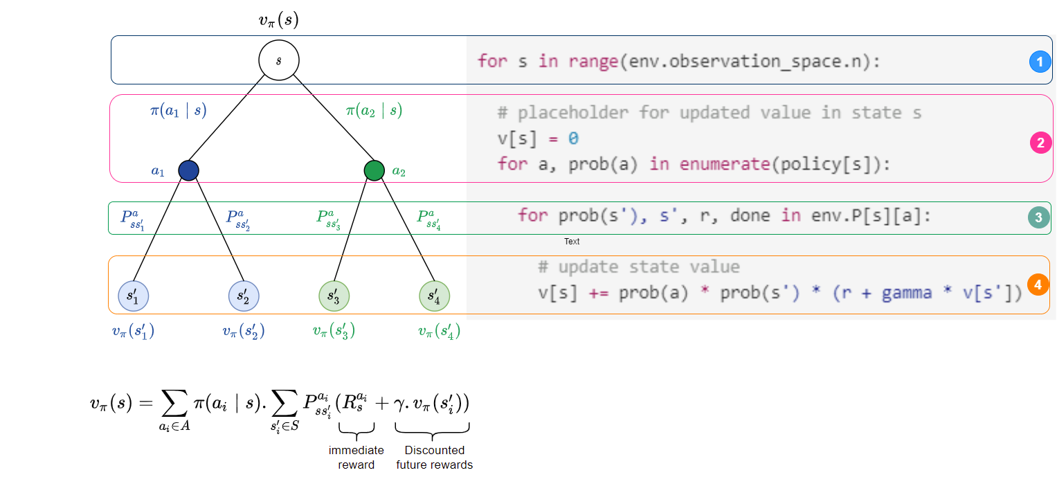
In the pseudocode above, prob(a) denotes the probability of action a (i.e. $\pi(a \mid s)$), s’ denotes the possible next state, and prob(s') denotes the transition dynamics (i.e. $P^{a}_{ss’}$).

Putting the above together in code:

def policy_eval(policy, env, gamma=0.9, th=1e-9, max_iter=10000):
    # number of iterations of evaluation
    eval_iter = 1
    # initialize the value function for each state
    v = np.zeros(env.observation_space.n)
    # repeat update until change in value is below th
    for i in range(int(max_iter)):
        # initialize change in value to 0
        delta = 0
        # for each state in env
        for st in range(env.observation_space.n):
            # initialize new value of current state
            v_new = 0
            # for each state s, 
            # v_new(s) = E[R_t+1 + gamma * V[s']]
            # average over all possible actions that can be taken from st
            for a, a_prob in enumerate(policy[st]):
                # v_new(s) = Sum[a_prob * nxt_st_prob * [r + gamma * v[s']]]
                # check how good the next_st is
                for nxt_st_prob, nxt_st, reward, done in env.P[st][a]:
                    # calculate bellman expectation
                    v_new += a_prob * nxt_st_prob * (reward + gamma * v[nxt_st])
                    
            # check to see if new state is better
            delta = max(delta, np.abs(v[st] - v_new))
            # update V
            v[st] = v_new
        eval_iter += 1
        
        # if value change is < th, terminate
        if delta < th:
            return v

The above function has some more details. It iteratively does it for a given max_iter number of iterations. Further, there is also an input threshold th which is used to decide when to stop updating the state value function v, by measuring the difference (delta) between the existing value and new value until it is negligible (as defined by th).

We have seen the benefits of deploying technology in many real world applications. Anyone who has used Yelp or IMDB or Rotten Tomatoes before deciding on a restaurant or watching a movie has accepted the indirect aid the (average) ratings on those sites provided about the quality of the restaurant or the movie. Anyone who has watched sports like Cricket, Tennis or Football (soccer) would be able to appreciate the role Hawk-Eye technology plays in resolving decision confusions by on-field referees or umpires. One just wonders how much of technology is used in other adjudications (like lawsuits, for example) and how technology can aid (rather than replace) such adjudications.

Let us take an example of such an adjudication - for example, a dispute between two parties (very much like two teams in a sport) being resolved by an adjudicator (like an on-field referee or an umpire).

In many sports, technology plays a huge role in aiding the on-field umpire or even over-turning the decisions of the on-field umpire when one of the parties was not satisfied with his original decision.

In cricket, this is referred to as Decision Review System (DRS) - which in turn uses several technologies like Hawk-Eye vision cameras, ball tracking technology and projection and estimation of the movement of the ball beyond the point of obstruction. How do we generalize this for any adjudication process.

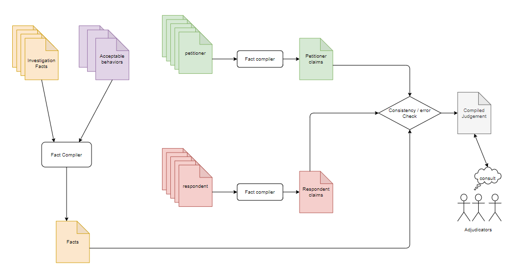
Shown below is a general flow of what a simplified process would look like.

Components of a Decision System

• Investigation Facts These are the facts coming out of an investigation. In sports, these could be coming from several cameras and ball tracking systems. In a civil or criminal lawsuit this could be the facts compiled by a set of investigators.

• Acceptable Behaviours These are the fair rules of the game. In sports, these could be coming from the rule book. In a lawsuit these could be the set of rules acceptable by law (and not necessarily by society).

• Fact Compiler is the brain of the system. It compiles the several statements in natural language into unambiguous statements in logic as a first step so that clear interpretation could be made. Then, a comparision of investigation facts against the rules of the game is made to see if all the rules were obeyed or some were not obeyed. The comparision tells us that happened that were actually allowed by the rules of the game (or by law) and what were disallowed by law.

Each of the two parties involved in the dispute can use such a Fact Compiler in order to compile their facts and check what was compromised and what rules were obeyed. There might be rule breaks that one party thinks was the right thing to do and needs an adjudicator to decide taking into account the situation under which the rule break happened (injuring another person during an act of self defence, for example).

Decision Systems Now, the decision making system has at least three sets of facts to compare - the compiled facts from each of the two parties involved in the dispute, and the fundamental truth compiled from independent investigation and acceptable (lawful) behaviours. The decision making system can compare these three sets of facts and enumerate the lawful and unlawful behaviours (w.r.t the truth as known to the investigation compared against acceptable legal behaviours). An adjudicator can consult this set of facts in order to avoid his own bias before making an adjudication. Purists might point out that this would not reduce bias as the bias introduced by investigation and fact compiler might indeed propagate to the compiled set of facts, and that is true. The effort to reduce the bias at these stages is to make the Fact Compiler and the input facts less biased by providing “more”, “unbiased” data.

Natural Language Understanding While understanding natural language with context is a challenging area of Computer Science and Mathematical logic, this would pave way for an interesting area of research to encode the contexts and use that encoding while building technologies to understand natural language. One of the simplest examples why this is a challenge is to just look at the following pairs of sentences (inspired by this)and guess an appropriate word for the blank in the second statement:

Time flies like an arrow
Fruit flies like a _______

Most AI systems would not guess the blank as a fruit, let alone one that rhymes with arrow (like mango). The word “like”, though the same word and spelling in both cases, alters the meaning of the statements that pure structural analysis would not help one in completing the second one. We need some semantics and context behind the statements. Another example would be to check if a given statement is a sarcastic one or a serious one. Sarcasm detection, though there are partially successful approaches, is a challenging area for natural language understanding systems.

Automated Reasoning Engines, Logic and Encoding Facts Many of the reasoning engines built for reasoning about the correct of computer programs (a set of program statements with a specific syntax (syntax of the programming language), much like the set of facts in English) work on predicate logic and there are well known automated solvers to solve a set of facts encoded in this logic. However, encoding contexts and possibilities would involve more than just predicate logic - it might involve modal logic and epistemic logic. A single reasoning engine would do the logical consistency check and derive the consequences (a set of facts) from known facts (provided by the supporting documents) based on encodings of rules of law (the axioms). Once the individual facts from investigations are compiled into precise mathematical statements by the Fact Compiler, rather than ambiguous English statements, the checker can be implemented using technologies behind reasoning engines used in program verification. While research in this area is progressing, it is also important to keep an eye on the applications - like lawsuits as legal statements in English language might require more effort to encode rather than informal statements in English language.

While aiding an adjudicator is an important part of the technology, encoding the facts, at each level of the process, as statements in mathematical logic would allow allow one to play back the compiled judgement (a set of facts) to understand how those facts were arrived at, from the initial sets of facts (like investigations and laws).

This would be a huge step in explaining the decision made (this would be the cornerstone of an explainable AI system). It would also provide a valuable tool for adjudicators to replay different decisions to check if they would be consistent with the initial sets of facts, or even replay them with some facts removed or altered to explain how the decision would have been different in case one of the parties had done something different (been more lawful instead of breaking the law).