-
Taking a Random Walk on a Frozen Lake →
In a previous post we played with OpenAI Gym on a simple example so that we can also manually workout and understand what is happening. Further the environment space, rewards, transition dynamics and transition probabilities were all clear (hopefully) from the simple example.
The end goal in Reinforcement Learning (RL) is to program our agent so that they interact with the environment and take decisions on their own and get better at reaching their goal on their own. When we say better we need to also mention what does better mean. It depends on the problem. For the 4x4 FrozenLake example we played with a better agent is one who can reach the
Gtile in shortest number of steps without falling intoH. The policy that gives the best is the optimal policy.What if we take random steps - at every time step, the agent can roll a die and decide which way to move - how many steps does that take to reach the goal (if at all it can be reached). We know that policy is a distribution of actions over states. We can initialize a policy
rand_policyrand_policy = np.ones([env.observation_space.n, env.action_space.n])where
env.observation_space.nandenv.action_space.nare the state spaces of observations and actions (16 and 4 for this example). We can write a simple function that would take a random step sampled from among the possible actions in the action space.env.step(env.action_space.sample())We maintain a counter and increment it until the goal state us reached or we fall into a hole, indicating the number of steps until an episode.
def rand_policy_eval():
    state = env.reset()
    cntr = 0
    done = False

    while not done:
        state, reward, done, info = env.step(env.action_space.sample())
        cntr += 1
    return cntr
We can plot and see how many steps an episode takes on an average.
rand_steps = [rand_policy_eval() for i in range(1000)]
print(f"Average number of steps to finish episode {np.mean(rand_steps)}")
sns.displot(rand_steps, kde=True)
plt.title('Distribution of random steps')
Average number of steps to finish episode 7.984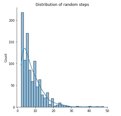
-
Bellman Expectation Equations - Action Value Function →
In a previous post we saw Bellman Expectation Equation for state value function $v_{\pi}(s)$. Following similar derivations, we can also derive Bellman Expectation Equation for the action value function $q_{\pi}(s, a)$.
Action value function $q_{\pi}(s, a)$ that denotes how good is it to take an action $a$ while being in state $s$
\[q_{\pi}(s, a) = \mathbb{E}_{\pi}[G_t \mid S_t = s, A_t = a]\]Since we know, from an earlier post that the return $G_t$ is the total discounted rewards starting from state s.
\[G_t = R_{t+1} + \gamma R_{t+2} + \cdots = \sum_{i=0}^{\infty} \gamma^{i} R_{t+i+1}\]Using the above in $q_{\pi}(s, a)$,
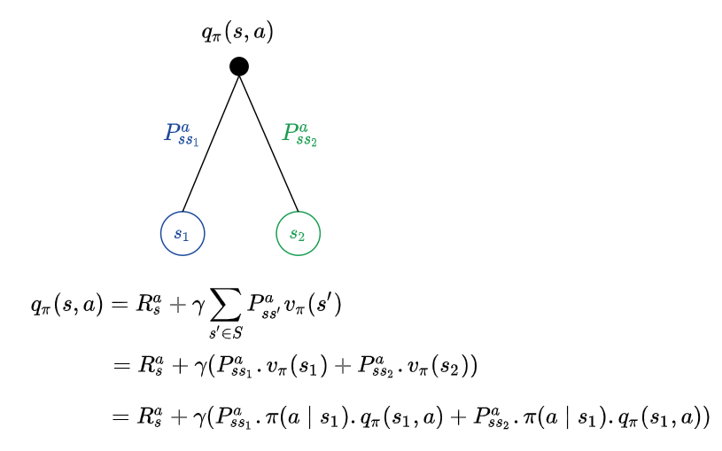
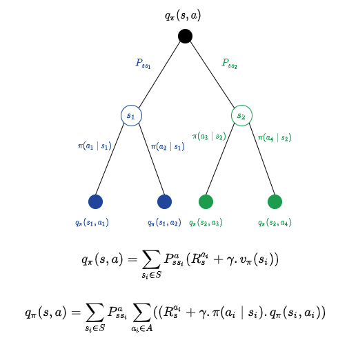
\[q_{\pi}(s, a) = \mathbb{E}_{\pi}[R_{t+1} + \gamma q_{\pi}(S_{t+1}, A_{t+1}) \mid S_t = s, A_t = a]\]Given a policy $\pi$, how good the action $a_1$ is would be known only by evaluating the action value function $q_{\pi}(s, a_1)$ for action $a_1$ while in state s , very analogous to evaluating the state value function $v_{\pi}(s)$ to evaluate how good the state s is. Suppose we have commited to an action a, the environment could react and take us to different states. Recall the earlier example, where we could have invested $300 in the stock market and the environment could have taken us to a state beneficial to us or to a state of despair. Formally, there could be different transitions possible out of our current state, with different transition probabilities, leading to different states. For example, an action a from state s could take us to state $s_1$ with probability $P_{ss_1}^{a}$ or to state $s_2$ with probability $P_{ss_2}^{a}$. When we are at a state where we have committed the action ($300 invested in stock) represented by the black filled circle, the value of the action would be the average of all the transition dynamics (as we do not know how the environment would react, yet).
Putting the state value function and action value function together,
Similarly, we could put the action value function and state value function together, as below.
This might look like lot many equations, but when we write an algorithm to implement these, we would use the equations as it is and hence these are very important to be understood.
-
OpenAI Gym - Playground for RL →
In some previous post we saw some theory behind reinforcement learning (RL). It is better to augment the theory with some practical examples in order to absorb the concepts clearly. While one can always get into some computer games and trying to build agents, observing the environment, taking some actions (game moves), it is worthwhile to start small and get an understanding of the many terminologies involved.
OpenAI provides OpenAI Gym that enables us to play with several varieties of examples to learn, experiment with and compare RL algorithms. We will see how to use one of the smallest examples in this post and map the terminologies from the theory section to the code fragments and return values of the gym toolkit.
We do the basic formalities of importing the environment, etc.
import gym
from gym import wrappers
from gym import envs
We shall look at ForestLake which is a game where an agent decides the movements of a character on a grid world.
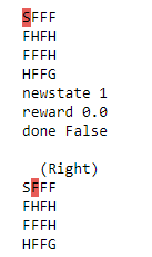
gym.make()creates the environment,reset()initializes it andrender()renders it.env = gym.make('FrozenLake-v1').env env.render()The rendered environment prints the following.

Some tiles in the grid are safe (marked
Ffor Frozen), while certain others (markedHfor Hole) lead to the agent falling into the lake. The tile markedSis supposed to be safe and the objective is to reach a tile markedGwhich is the agent’s goal, without falling into a hole.We will work with a small 4x4 grid so that it is easy to imagine the different states and compute actions and their results manually while we do it algorithmically. OpenAI gym offers a way to render the environment to see how the grid world looks like
We can also print the action space (the set of all possible actions) and the state space (the set of all possible states).
env.reset()
print('Action space {}'.format(env.action_space))
print('State space {}'.format(env.observation_space))
returns
Action space Discrete(4)
State space Discrete(16)
There are 4 possible actions - Left, Down, Right and Up and (corresponding to numbers 0, 1, 2 and 3). There are 16 possible states as it is a 4x4 grid (the agent can be on any tile on this grid). The agent is rewarded 0 points at each tile step for finding a path to
Gwithout encountering a hole. When it reachesGthe agent is rewarded 1 point.The transition dynamics for different actions can be obtained by looking at the transition table
P.env.P[0]prints
{0: [(0.3333333333333333, 0, 0.0, False), (0.3333333333333333, 0, 0.0, False), (0.3333333333333333, 4, 0.0, False)], 1: [(0.3333333333333333, 0, 0.0, False), (0.3333333333333333, 4, 0.0, False), (0.3333333333333333, 1, 0.0, False)], 2: [(0.3333333333333333, 4, 0.0, False), (0.3333333333333333, 1, 0.0, False), (0.3333333333333333, 0, 0.0, False)], 3: [(0.3333333333333333, 1, 0.0, False), (0.3333333333333333, 0, 0.0, False), (0.3333333333333333, 0, 0.0, False)]}env.P[state]($P_s$) is a tuple of the form:{action: [probability (next_state), next_state, reward, done]}i.e.
\[P_{s}^{a} = P_{s'}, s', r, done\]done indicates the completion of the episode (reaching
G). We see that from state 0 none of the actions we take would lead us toGand hence done isFalsefor all the actions. We take an action by callingenv.step(action)which returns a tuple of the form:print(env.P[14])prints
{0: [(0.3333333333333333, 10, 0.0, False),
     (0.3333333333333333, 13, 0.0, False),
     (0.3333333333333333, 14, 0.0, False)],
 1: [(0.3333333333333333, 13, 0.0, False),
     (0.3333333333333333, 14, 0.0, False),
     (0.3333333333333333, 15, 1.0, True)],
 2: [(0.3333333333333333, 14, 0.0, False),
     (0.3333333333333333, 15, 1.0, True),
     (0.3333333333333333, 10, 0.0, False)],
 3: [(0.3333333333333333, 15, 1.0, True),
     (0.3333333333333333, 10, 0.0, False),
     (0.3333333333333333, 13, 0.0, False)]}
We can see that some of the actions take us from state
14to the final state15and hence the valueTruefor done for such cases and the probability of $s’$ is also 1.0.{new_state, reward, done, info}For example,
env.reset()
env.render()
new_state, r, done, info = env.step(2)
print('newstate {}'.format(new_state))
print('reward {}'.format(reward))
print('done {}'.format(done))
print()
env.render()
returns
-
Bellman Expectation Equations - State Value Function →
In a previous post, we briefly introduced Bellman Expectation Equation and Bellman Optimality Equation. Let us recall the first of the two main functions state value function that we would be working with.
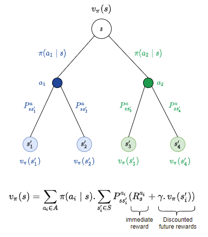
State value function $v_{\pi}(s)$ that denotes how good is it to be in state $s$ following policy $\pi$
\[v_{\pi}(s) = \mathbb{E}_{\pi}[G_t \mid S_t = s]\]Since we know, from an earlier post that the return $G_t$ is the total discounted rewards starting from state s.
\[G_t = R_{t+1} + \gamma R_{t+2} + \cdots = \sum_{i=0}^{\infty} \gamma^{i} R_{t+i+1}\]Using the above in $v_{\pi}(s)$,
\[v_{\pi}(s) = \mathbb{E}_{\pi}[R_{t+1} + \gamma v_{\pi}(S_{t+1}) \mid S_t = s]\]Since a policy $\pi$ is a distribution of actions over states, from each state s we will have different actions with different probabilities. We might take an action $a_1$ to invest 300 in stock market and at that point we are committed to that action $a_1$. The environment (which might only be partially observable) might react in such a way as to create a market crash or it might reach in such a way as to boost our profits.
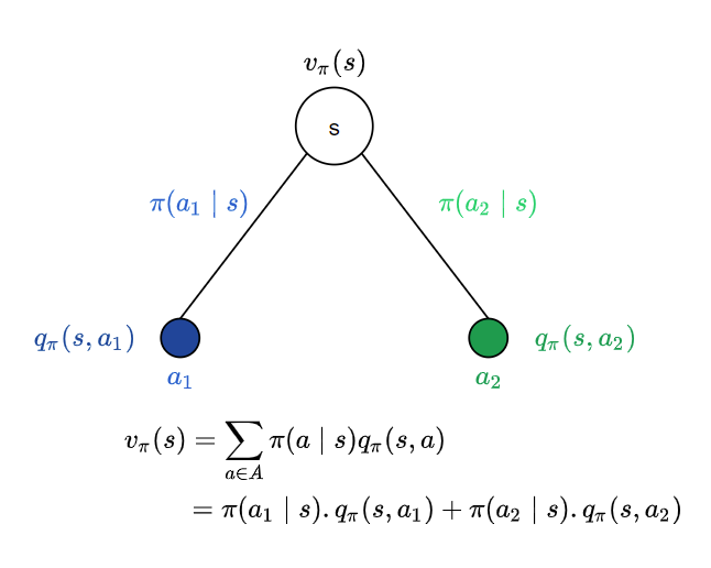
Following policy $\pi$, from state s, we have two possible actions $a_1$ and $a_2$ with probabilities $\pi(a_1 \mid s)$ and $\pi(a_2 \mid s)$. From the point of view of state s, the value of the state is the average over all possible actions we could take from state s, following policy $\pi$. In this case we have two actions and hence it would be the average over these two. Since the probability of an action $a_i$ is $\pi(a_i \mid s)$ and the outcome is the value of action $a_i$ given by the action value function $q_{\pi}(s, a_i)$ the expectation is $\pi(a_i \mid s) . q_{\pi}(s, a_i)$
Each of these actions might lead us to different sequences of states depending on how the environment reacts. We will see how to formulate this in a future post.
-
Reinforcement Learning - Value, Policy and Action →
In a previous post, we looked at some more terminology in order to dive into Reinforcement Learning (RL). We will see some more key constituents of RL in this one. In particular, we will see how we evaluate states and policies and how actions play a role.
We already saw that states are evaluated using state value function - v(s) that tells us how good a state s is. We also know that our agent can decide to take certain actions to move from one state to another. The agent, ideally, should take the best action - the one that would maximize the value of the states the agent would end up in, by taking the action(s). We talked about an example of taking two actions that correspond to spending $300 in two different ways. Since there could be multiple actions with different probabilities, each action would lead to a different outcome. What determines the actions we take? Are there rules that allow us to decide?
A policy denoted by $\pi$ is a distribution of actions over states, i.e. it denotes the probabilities of different actions given a state s. This completely defines the behavior of the agent. The agent uses a policy to decide what actions to take. Hence in RL, we need to identify the best policy - that would lead us to states with maximum returns. More formally,
\[\pi(a \mid s) = \mathbb{P}[A_t = a \mid S_t = s]\]Given a policy $\pi$ the transition dynamics defined by our Markov process would take us through a sequence of states that would get us rewards for that policy. Since actions help us transition from one state to another, the overall transition dynamics (it is after all a probabilistic system and each action has a specific probability of being taken) would be the average of all the actions that take us through the different sequences of states. More formally,
\[\mathcal{P}^{\pi}_{s, s'} = \sum_{a \in A} \pi(a \mid s)\mathcal{P}_{s, s'}^{a}\]The rewards would therefore be,
\[\mathcal{R}_{s}^{\pi} = \sum_{a \in A} \pi(a \mid s)\mathcal{R}^{a}_{s}\]Given a policy $\pi$, we can encapsulate all the knowledge we need in two functions:
- State value function $v_{\pi}(s)$ that denotes how good is it to be in state $s$ following policy $\pi$
- Action value function $q_{\pi}(s, a)$ that denotes how good is it to take an action $a$ while being in state $s$
Stepping back from formalizing, let us rething what is our ultimate goal when we program an agent. We want to:
- Identify what are the best states to be in (with the help of state value function)
- Identify what action to choose whatever state we end up in (with the help of action value function)
But we are not just satisfied by knowing how good a state is or even how good an action in a given state is. We want to find the best (optimal) values for state value function and action value functions - denoted by $ v_* (s)$ and $ q_* (s, a)$ over all possible policies. These are governed by two equations:
- Bellman Expectation Equation - that helps us with evaluating states and actions
- Bellman Optimality Equation - that helps us in identifying optimal states and actions
The formalisms we came up in this and in the previous post would help us arrive at the above equations.