Bellman Expectation Equations - State Value Function →
In a previous post, we briefly introduced Bellman Expectation Equation and Bellman Optimality Equation. Let us recall the first of the two main functions state value function that we would be working with.
State value function $v_{\pi}(s)$ that denotes how good is it to be in state $s$ following policy $\pi$
\[v_{\pi}(s) = \mathbb{E}_{\pi}[G_t \mid S_t = s]\]Since we know, from an earlier post that the return $G_t$ is the total discounted rewards starting from state s.
\[G_t = R_{t+1} + \gamma R_{t+2} + \cdots = \sum_{i=0}^{\infty} \gamma^{i} R_{t+i+1}\]Using the above in $v_{\pi}(s)$,
\[v_{\pi}(s) = \mathbb{E}_{\pi}[R_{t+1} + \gamma v_{\pi}(S_{t+1}) \mid S_t = s]\]Since a policy $\pi$ is a distribution of actions over states, from each state s we will have different actions with different probabilities. We might take an action $a_1$ to invest 300 in stock market and at that point we are committed to that action $a_1$. The environment (which might only be partially observable) might react in such a way as to create a market crash or it might reach in such a way as to boost our profits.
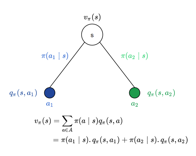
Following policy $\pi$, from state s, we have two possible actions $a_1$ and $a_2$ with probabilities $\pi(a_1 \mid s)$ and $\pi(a_2 \mid s)$. From the point of view of state s, the value of the state is the average over all possible actions we could take from state s, following policy $\pi$. In this case we have two actions and hence it would be the average over these two. Since the probability of an action $a_i$ is $\pi(a_i \mid s)$ and the outcome is the value of action $a_i$ given by the action value function $q_{\pi}(s, a_i)$ the expectation is $\pi(a_i \mid s) . q_{\pi}(s, a_i)$
Each of these actions might lead us to different sequences of states depending on how the environment reacts. We will see how to formulate this in a future post.