Temperature and Sampling in LLMs →
The original motivation for using temperature to control the output of Large Language Models (LLMs) comes from Statistical Mechanics. This concept was adopted for neural networks probably first by David Ackley, Geoffrey Hinton and Terrence Sejnowskli in A Learning Algorithm for Botzmann Machines. While the paper talks about constraint satisfaction problems using a parallel network of processing units, the way to understand the concept of temperature for today’s neural networks is simpler.
Think of the neural network structure given below:
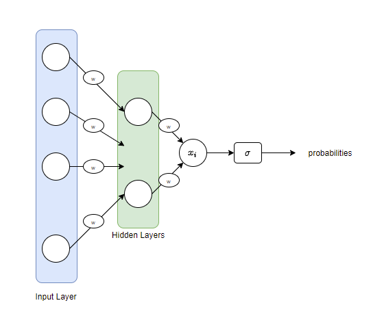
We have an Input layer, a set of hidden layers and also the activations shown by w (for multiplication by weight elements). What we get as an output is a real value $x_i$. If we are dealing with a binary classification task, what we want is to interpret this value $x_i$ to have two probabilities indicating the probabilities for the two possible classes. If our task is a multi-class classification, we will have more probabilities for outputs. A common choice for this is a sigmoid function, which for binary classification tasks is the logistic function and in multi-class tasks, the multinomial logistic function (softmax). This is the primary reason behind books referring to the arguments of softmax as logits. The term logit was originally used by Joseph Berkson to mean log of odds and as an analogy for probit.
Let’s understand it using some simple code fragments. In the below, we have some probabilities probs that add up to 1.
probs = [0.0001, 0.0179, 0.002, 0.03, 0.05, 0.4, 0.5]
probs, sum(probs)

> ([0.0001, 0.0179, 0.002, 0.03, 0.05, 0.4, 0.5], 1.0)
Let us calculate the log of the odds of these.
import math

def get_logits(probs):
  return [math.log(x/(1-x)) for x in probs]

logits = get_logits(probs)
logits

> [-9.21024036697585,
 -4.00489242331702,
 -6.212606095751519,
 -3.4760986898352733,
 -2.9444389791664403,
 -0.4054651081081643,
 0.0]
Let us compute the regular softmax function:
\[\sigma(x_i) = \frac{e^{x_i}} {\sum\limits_{i} e^{x_i}}\]def softmax(logits):
denominator = sum([math.exp(x) for x in logits])
softmax = [math.exp(x)/denominator for x in logits]
return softmax
And compute the softmax for our logits - essentially we are converting them into an interpretable way.
softmax(logits)

> [5.648507096749673e-05,
 0.010294080664302612,
 0.0011318521535150297,
 0.017467862616618552,
 0.029726011821263155,
 0.37652948306933326,
 0.5647942246039999]
Now, let us add the temperature parameter to control the softmax output. Our modified softmax is now:
\[\sigma(x_i) = \frac{e^{\tfrac{x_i}{T}}}{\sum\limits_{i} e^{\tfrac{x_i}{T}}}\]def softmax_t(logits, t=1.0):
denominator = sum([math.exp(x/t) for x in logits])
softmax = [math.exp(x/t)/denominator for x in logits]
return softmax
If we now compute softmax for different values of temperature (t in the function above),
softmax_t(logits, t=0.1)

> [9.83937567458523e-41,
 3.976549800632757e-18,
 1.0268990926840024e-27,
 7.870973150024767e-16,
 1.6032351163946892e-13,
 0.017045927454927112,
 0.9829540725449118]
For small temperature values t=0.1 for example, we see that the smaller logits almost vanish and the larger ones survive. If you think of these as tokens in the target language (a source-target language translation or content generation in a target language), it would mean that only a few of the tokens get a chance to be used and hence it would be relatively bland content.
If we increase the temperature, say to a 1 (t=1):
softmax_t(logits, t=1)

> [5.648507096749673e-05,
 0.010294080664302612,
 0.0011318521535150297,
 0.017467862616618552,
 0.029726011821263155,
 0.37652948306933326,
 0.5647942246039999]
If we keep increasing it to a 100, and then to a 1000, we see more interesting behaviors.
softmax_t(logits, t=100)

> [0.13520713120321545,
 0.14243152917854485,
 0.13932150536327115,
 0.14318669304928164,
 0.1439499862705803,
 0.14765163186672028,
 0.14825152306838635]

softmax_t(logits, t=1000)

> [0.14207868212056274,
 0.1428201792975013,
 0.14250522103172697,
 0.14289572168473877,
 0.1429717137819637,
 0.143335176443405,
 0.14339330564010144]
We see that more tokens are having similar chances of getting used. In the above case, at t=1000, every token has equal probability of getting used in the target language and hence it has more creative freedom to use all possible words and create more previously unseen (and some times awkward) content.